AVERY_BOOKS // NUCLEAR

// SECTION_01 :: PROJECT_STAGES

STAGE_01 IN_PROGRESS

Grid Geometry & Ion-Dynamics Simulation

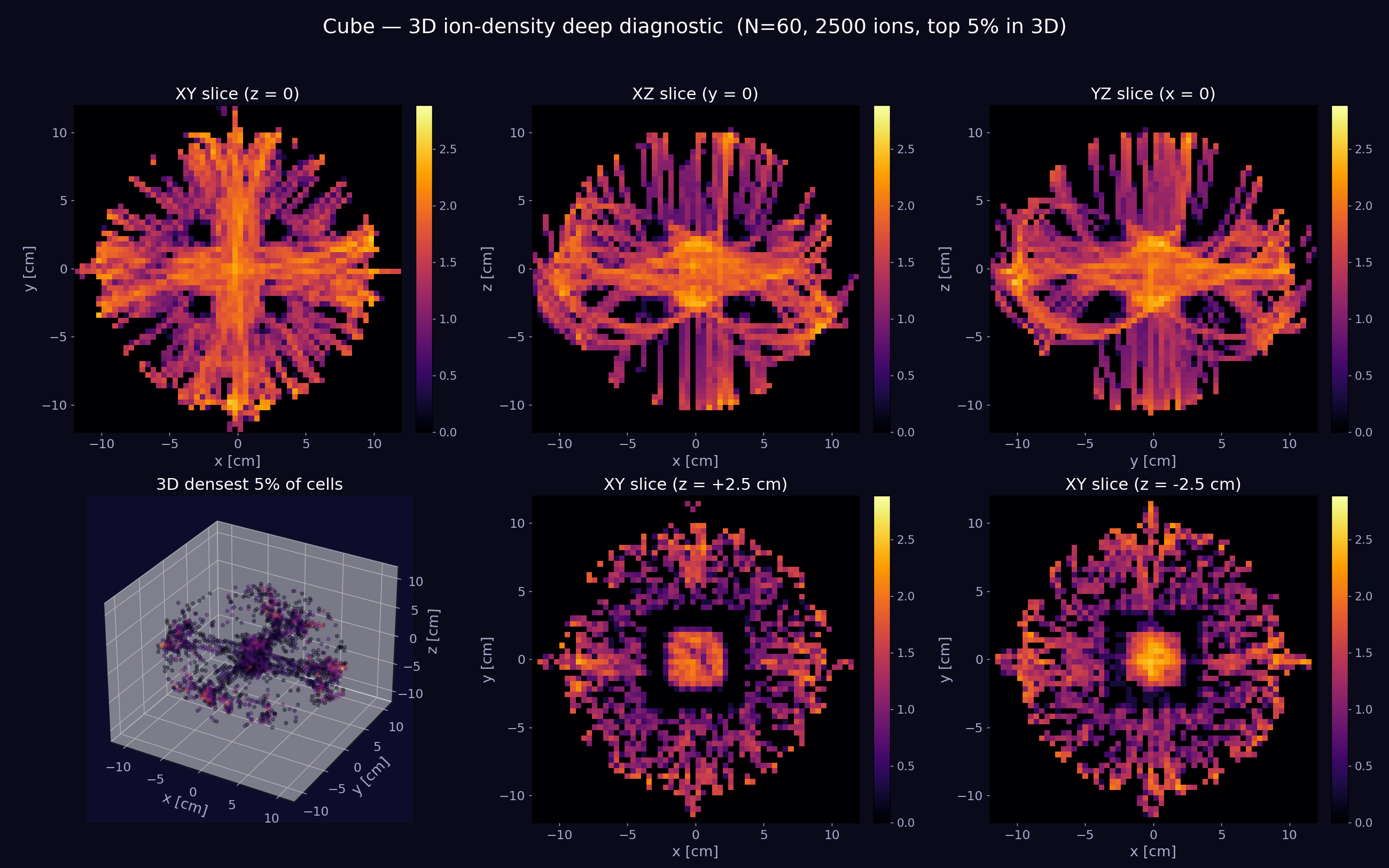
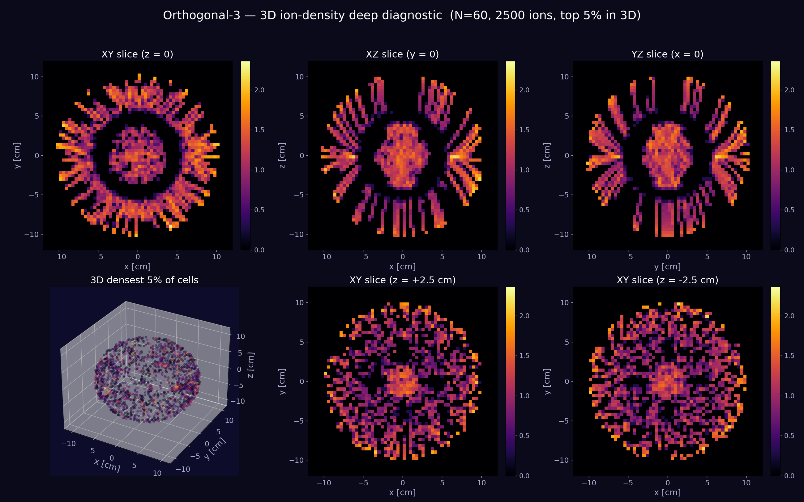
Simulating electric potential via Poisson/Laplace solvers with Dirichlet boundary conditions, and modeling ion density / dynamics across candidate grid geometries to select an optimal confinement configuration.

STAGE_02 PLANNED

Fusor Construction & Spectroscopy Rig

Build the physical fusor, high-voltage supply, and a Raspberry-Pi optical spectroscopy rig.

STAGE_03 PLANNED

Plasma Behavior Diagnostics

Characterize and classify plasma behaviors via optical spectroscopy and diagnostics.

// SECTION_02 :: RESULTS

Cube grid ion density distribution — The cube grid results in a well defined 6-jet structure with clean kinematic behavior. The beams are well-collimated along each cartesian axis. The ion density is slightly stronger in the XY plane, and the Z axis jets are slightly weaker. The jet structure does not have the symmetry that Able inversion requires, so radial profiles are not applicable. Therefore this grid is best suited for velocity space analysis, not spatial analysis.

Orthogonal grid ion density distribution — The orthogonal grid results in a mostly radially symmetric ion density distribution, with small jets forming along the principal axes. The core maintains symmetry for Abel inversion, which can allow for spectral confirmation that confinement is occurring. It also does not have strong enough ion escape beams to interfere with longer integrations of the core in spectroscopy. This will allow for contamination, SNR, and temperature ratios to occur. The symmetry and line of sight clarity of the spherical grid makes it most suitable for spatial analysis of core plasma characteristics.

// SECTION_03 :: PHYSICS_DISCUSSION

Inertial Electrostatic Confinement

Inertial Electrostatic Confinement (IEC) is a method of plasma confinement that uses electric fields and potential wells to accelerate ions towards a central region, where they can collide and potentially undergo nuclear fusion. The fusor design typically consists of two concentric spherical grids: an outer grid that is grounded and an inner grid that is negatively charged. Ions are drawn towards the center, where they gain kinetic energy and can collide with other ions. The effectiveness of IEC depends on factors such as grid geometry, voltage applied, and ion density.

Potential Well & Grid Geometry

Grid geometry is crucial in determining the shape and depth of the potential well created by the fusor. Typical grid geometries include spherical, toroidal, cubic, and octahedral configurations. More symmetric and spherical geometries tend to produce more uniform cores, where grids with defined sides produce stronger jets along the normal to the grid faces. So octahedral grids have some level of anisotropy compared to spherical grids. Custom grid geometries are also possible, which find a balance between core symmetry and jet control.

Plasma Diagnostics

Plasma diagnostics are essential for understanding the behavior of the plasma within the fusor. Techniques such as optical spectroscopy, Langmuir probes, and interferometry can provide insights into plasma density, temperature, and composition. By analyzing the emitted light from the plasma, researchers can determine the energy levels of ions and electrons, as well as identify any impurities present. These diagnostics help in optimizing the fusor's performance and achieving better confinement.
This project will focus on optical spectroscopy using a Raspberry Pi based camera. It will focus on using Doppler broadening to determine the temperature of the plasma, and using line ratios to determine the density of the plasma. It will also focus on long term integration of the plasma to determine the stability of the plasma over time, and to determine if the plasma is in a steady state or if it is oscillating.

// SECTION_04 :: CODE_DISCUSSION

Simulation Code // numerical methods

The Stage-1 simulation runs on two numerical kernels: a Poisson/Laplace solver that builds the electrostatic field from the grid geometry, and a Boris integrator that pushes ions through that field.

Poisson solver & Dirichlet boundary conditions

The potential φ satisfies Poisson's equation ∇²φ = −ρ/ε₀ (Laplace's ∇²φ = 0 in the charge-free gaps between electrodes). The grid wires are Dirichlet boundaries, where their voltage is fixed (cathode at −30 kV, grounded chamber at 0 V) and re-pinned every sweep. On a uniform 3-D mesh the Laplacian becomes the 7-point finite-difference stencil, relaxed with Gauss–Seidel and successive over-relaxation until the field stops changing.

# 7-point finite-difference Poisson update (Gauss-Seidel + SOR)
for it in range(max_iter):
    phi_old = phi.copy()
    phi[1:-1, 1:-1, 1:-1] = (1 - w) * phi[1:-1, 1:-1, 1:-1] + w * (
        phi[2:, 1:-1, 1:-1] + phi[:-2, 1:-1, 1:-1] +
        phi[1:-1, 2:, 1:-1] + phi[1:-1, :-2, 1:-1] +
        phi[1:-1, 1:-1, 2:] + phi[1:-1, 1:-1, :-2] +
        rho[1:-1, 1:-1, 1:-1] * dx * dx / eps0
    ) / 6.0
    phi[grid_mask] = grid_voltage          # Dirichlet BC: re-pin electrodes
    if np.max(np.abs(phi - phi_old)) < tol:
        break
E = -np.gradient(phi, dx)                   # field used by the ion push

Boris algorithm (ion push)

Ion trajectories are advanced with the Boris integrator, the standard leapfrog pusher for charged particles. Each step splits the Lorentz force into a half electric kick, a magnetic rotation, then a second half electric kick. The rotation conserves speed, so the scheme is time-reversible and energy-stable over the many core recirculations an ion makes (here B ≈ 0, so the electric half-kicks dominate).

# Boris push: advance velocity v, then position x
qmdt2 = (q / m) * (dt / 2)
v_minus = v + qmdt2 * E                     # half electric kick
t = qmdt2 * B                               # magnetic rotation vector
s = 2 * t / (1 + np.dot(t, t))
v_prime = v_minus + np.cross(v_minus, t)
v_plus  = v_minus + np.cross(v_prime, s)
v = v_plus + qmdt2 * E                      # second half electric kick
x = x + v * dt                              # drift

NUCLEAR_FUSOR